Epilogue

Congratulations, and thank you for going through this book. As I have said in the preface, linear algebra is a universal prerequisite for most mathematics. This also means that once you become familiar with linear algebra, there are many directions in which you can proceed. I would like to discuss what advanced mathematics one can learn having digested linear algebra.

Calculus in higher dimensions

We will assume that the reader already knows calculus in a single variable. To do calculus in many variables, we can simply use $\mathbb{R}^n$, but let me introduce the concept of a manifold.

Imagine being a physicist. You are faced with the problem of modeling the universe. Everyone knows that there are three linearly independent directions in which we can move. So the natural candidate for the universe is $\mathbb{R}^3$. But you look back and think about the age when people thought the Earth is flat. Well, you can walk in two linearly independent directions at any point on Earth, but $\mathbb{R}^2$ turns out to be a terribly wrong model. Why can't this happen for the universe?

Of course this is a non-rigorous description, but it captures an important idea that we only want a space to locally look like Euclidean space. Let us look at a few examples. The circle

$$ S^1 = \lbrace (x, y) : x^2 + y^2 = 1 \rbrace $$

is a $1$-manifold. The set

$$ X = [-1, 1] \times \lbrace 0\rbrace \cup \lbrace 0\rbrace \times [-1, 1] \subseteq \mathbb{R}^2 $$

is not, because near $(0, 0)$ it doesn't look like a line. The doughnut

$$ T^2 = \lbrace (x, y, z) : z^2 + (\sqrt{x^2 + y^2} - 1)^2 = 0.5 \rbrace \subseteq \mathbb{R}^3 $$

is a $2$-manifold.

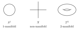
The circle is labeled a one-manifold, the crossing of two line segments is labeled a non-manifold, and the torus is labeled a two-manifold.

Let us now fix an $n$-dimensional manifold $M$ and consider an infinitely differentiable function $f : M \to \mathbb{R}$. Let us think about how we may define the derivative $df$ of $f$. When $M = \mathbb{R}$, the derivative $f^\prime$ was defined as

$$ f^\prime(x) = \lim_{\Delta x \to 0} \frac{f(x + \Delta x) - f(x)}{\Delta x}. $$

But for a general manifold $M$, what does $\Delta x$ mean? It should be an infinitesimal displacement of $x$, so that $x + \Delta x$ is a point very close to $x$. So we take $\Delta x$ to be a tangent vector to the manifold at $x$.

It is difficult to precisely describe what a tangent vector is, but it should be considered as a “direction” with which a point can move, also remembering the “speed”. A tangent vector defines a differential operator by taking the difference quotient,

$$ D_v(f) = \lim_{\epsilon \to 0} \frac{f(p + \epsilon v) - f(p)}{\epsilon}. $$

This is sometimes called the directional derivative of $f$.

If we denote by $C_\infty(M)$ the vector space of infinitely differentiable functions on $M$, then the $\mathbb{R}$-linear functional $D_v : C^\infty(M) \to \mathbb{R}$ can be considered a differential operator. It is characterized by satisfying the Leibniz identity

$$ D_v(fg) = D_v(f) g(p) + f(p) D_v(g). $$

The set of tangent vectors at a fixed point $p \in M$ naturally forms an $n$-dimensional $\mathbb{R}$-vector space (by $D_{v+w} = D_v + D_w$ and $D_{cv} = c D_v$), and this vector space $T_p M$ is called the tangent space of $M$ at $p$.

So given a function $f \in C_\infty(M)$ (i.e., a function $f : M \to \mathbb{R}$), we get a linear map

$$ df \vert_p : T_p M \to \mathbb{R}; \quad v \mapsto D_v(f). $$

That is, for each point $p \in M$, we get an element of the dual tangent space $T_p^\ast M = (T_p M)^\ast$, also called the cotangent space. This assignment to each point $p \in M$ an element of $T_p^\ast M$ is called a $1$-form.

Using the language of $1$-forms, we can also formulate the fundamental theorem of calculus. Consider a curve $\gamma$ in $M$, which is a smooth function $\gamma : [a, b] \to M$ for some interval $[a, b] \subseteq \mathbb{R}$. Then for a partition $a = a_0 < a_1 < \cdots < a_{k-1} < a_k = b$, we can write

$$ f(\gamma(b)) - f(\gamma(a)) = \sum_{i=0}^{k-1} \bigl(f(\gamma(a_{i+1})) - f(\gamma(a_i))\bigr) \approx \sum_{i=0}^{k-1} (df) (\gamma(a_{i+1}) - \gamma(a_i)), $$

where the summand is evaluating the “tangent vector” $\gamma(a_{i+1}) - \gamma(a_i)$ at $df$. As $\max_{i} (a_{i+1} - a_i) \to 0$. The right hand side can be adequately interpreted as the integral $\int_{\gamma} df$. Then the equation can be rewritten as

$$ f(\gamma(b)) - f(\gamma(a)) = \int_{\gamma}^{} df. $$

There even is a higher-dimensional analogue of the fundamental theorem of calculus. This is now a bit complicated to explain, and hence we will only state the theorem without any explanation.

So a $0$-form is just a function $f : M \to \mathbb{R}$, and a $1$-form is an assignment to each $p \in M$ an element $\omega_p \in T_p^\ast M$. It turns out there is a way to take an arbitrary $k$-form $\omega$ and take its derivative to get a $(k+1)$-form $d\omega$.

Consider the case when $n = 1$ and $M = [a,b]$. The differential form $\omega = f$ is a $0$-form, which is a function, and the boundary of $M$ consists of the two points $a$ and $b$. In this case, the integral of $f$ over the two points is $f(b) - f(a)$ and the right hand side is just $\int_{[a,b]}^{} df$. So we recover the fundamental theorem of calculus.

• For calculus with a single variable, there is Rudin's classic textbook Principles of Mathematical Analysis, which provides a rigorous and comprehensive introduction to analysis. It starts from scratch and also develops multivariable calculus near the end.

• There is a series of books on multivariable calculus written by Spivak. There is Calculus on Manifolds, which leads up to Stokes's theorem in the context of manifolds. There also is the more advanced book A Comprehensive Introduction to Differential Geometry, Volume One that discusses the topic in a geometric manner.

• Lee's Introduction to Smooth Manifolds contains almost the same material as in Spivak's A Comprehensive Introduction, but takes a differential topology perspective.

Representation theory

The Frobenius normal form, Jordan normal form, and related theorems convey information about the possible ways a linear map can act on a finite-dimensional vector space. More precisely, they tell us that we can find a suitable basis such that the linear map takes a certain form.

But what if there are many linear maps, and some of them have a certain relation they need to satisfy? To elucidate what I am trying to say, let us make a definition.

Here is an example. Take the set $\mathbb{Z}$ with $\mu(x, y) = x + y$. One can readily check that it is a group. Here is a slightly more complicated example. Consider

$$ S_n = \lbrace (f : \lbrace 1, \ldots, n\rbrace \to \lbrace 1, \ldots, n\rbrace ) \text{ bijective} \rbrace $$

with composition as multiplication. For instance, $\tau \in S_3$ is defined as $\tau(1) = 2$, $\tau(2) = 1$, $\tau(3) = 3$, and $\sigma \in S_3$ is defined as $\sigma(1) = 2$, $\sigma(2) = 3$, $\sigma(3) = 1$, then we have the identities

$$ \tau^2 = 1, \quad \sigma^3 = 1, \quad \tau \sigma \tau = \sigma^2. $$

Once we have a group $G$, such as $G = S_3$, we might want to represent it as a matrix. For instance, if we associate

$$ \tau = \begin{bmatrix} 0 & 1 \\ 1 & 0 \end{bmatrix}, \quad \sigma = \begin{bmatrix} 0 & -1 \\ 1 & -1 \end{bmatrix}, $$

then the identities $\tau^2 = 1$, $\sigma^3 = 1$, $\tau \sigma \tau = \sigma^2$ are all satisfied.

If $(V_1, \rho_1)$ and $(V_2, \rho_2)$ are both representations of a group $G$, we can form the direct sum $V_1 \oplus V_2$, and the representation

$$ (\rho_1 \oplus \rho_2)(g) = \rho_1(g) \oplus \rho_2(g). $$

It can be easily checked that this construction gives a representation of $G$.

Representations of finite groups over $k = \mathbb{C}$ have a nice characterization. First of all, all representations can be written as a direct sum of irreducible representations. This means that to study representations, it is enough to study irreducible representations. Here is the big theorem.

Let me demonstrate the theorem with the group $S_3$. There are three equivalence classes for $g \sim h g h^{-1}$,

$$ \lbrace e \rbrace , \quad \lbrace \sigma, \sigma^2 \rbrace , \quad \lbrace \tau, \sigma \tau, \sigma^2 \tau \rbrace . $$

Then there should be three irreducible representations. These are

$$ \begin{aligned} \rho_1(\tau) &= \begin{bmatrix} 1 \end{bmatrix}, & \rho_1(\sigma) &= \begin{bmatrix} 1 \end{bmatrix}, \\ \rho_2(\tau) &= \begin{bmatrix} -1 \end{bmatrix}, & \rho_2(\sigma) &= \begin{bmatrix} 1 \end{bmatrix}, \\ \rho_3(\tau) &= \begin{bmatrix} 0 & 1 \\ 1 & 0 \end{bmatrix}, & \rho_3(\sigma) &= \begin{bmatrix} 0 & -1 \\ 1 & -1 \end{bmatrix}. \end{aligned} $$

And we have $1^2 + 1^2 + 2^2 = 6$, which is the size of the group.

This theorem pretty much tells us everything about finite-dimensional representations of finite groups over $\mathbb{C}$. A more interesting topic to study is representations of Lie groups or of Lie algebras.

Let us take $S^1$ for example. We may identify $S^1$ with the unit complex numbers.

$$ S^1 \quad \leftrightarrow \quad \lbrace z \in \mathbb{C} : \lvert z \rvert = 1 \rbrace $$

Then $S^1$ naturally has a multiplicative structure, and it can be easily verified that this is a group. Another example is

$$ \operatorname{SU}(2) = \lbrace 2 \times 2 \text{ complex matrices } U \text{ such that } U U^\dagger = U^\dagger U = I \text{ and } \det U = 1 \rbrace . $$

Because the product of unitary matrices is unitary, and the determinant is multiplicative, this is a group. It is harder to show that $\operatorname{SU}(2)$ is a manifold, but it turns out that $\operatorname{SU}(2) \cong S^3$.

We might ask what are the finite-dimensional irreducible representations of $\operatorname{SU}(2)$ over $\mathbb{C}$. It turns out that there is a nice answer to this.

Such a nice description exists when the Lie group $G$ is compact.

• For an introduction with many concrete examples, take a look at Fulton and Harris's Representation Theory: A First Course. The book starts with the representation theory of finite groups at the beginning, and later also discusses Lie groups and Lie algebras.

• There is also Introduction to Representation Theory written by Etingof et al., which is legally freely available on the internet. This book also begins with representation theory of finite groups, but delves into the combinatorial aspects of representations instead of Lie algebras.

• Kirillov's book Introduction to Lie Groups and Lie Algebras focuses on Lie algebras, Lie groups, and their representations. A preliminary version of the book is available for free from the author's website.

Functional analysis

In Chapter 5, we talked about finite-dimensional Hilbert spaces in detail. But we alluded that there is a notion of an infinite-dimensional Hilbert space.

Here is an example. Consider the space

$$ C^0(S^1) = \lbrace (f : \mathbb{R} \to k) \text{ continuous} : f(x) = f(x+1) \text{ for all } x \in \mathbb{R} \rbrace , $$

and the inner product

$$ \langle f, g \rangle = \int_{0}^{1} \overline{f(x)} g(x) dx. $$

This is an inner product space that is infinite-dimensional, but it does not satisfy (H1). So we “complete” the vector space by adding in vectors if a Cauchy sequence does not converge. Define

$$ L^2(S^1) = \text{completion of } C^0(S^1) \text{ with respect to the } L^2\text{-norm}. $$

This satisfies (H1) by construction, and it also satisfies (H2) because the set of piecewise linear functions with rational slopes and bending points is both dense and countable.

For Hilbert spaces, many of the theorems we discuss hold.

There is also a spectral theorem in this context. However, we need a somewhat restrictive condition to make the proof work.

Although such a theorem seems satisfactory from a theoretic point of view, it is not very useful when doing analysis. We said that the differential operator $T : \frac{\partial^2}{\partial x^2}$ is roughly a self-adjoint operator because integration by parts gives

$$ \int_{}^{} \bar{f}^{\prime\prime} g = -\int_{}^{} \bar{f}^\prime g^\prime = \int_{}^{} \bar{f} g^{\prime\prime}. $$

In the attempt to apply the spectral theorem to this operator, the first problem we encounter is that $T : L^2(S^1) \to L^2(S^1)$ is not really defined on the entire domain. A function has to be twice-differentiable for its image under $T$ to be defined. This is closely related to the fact that $T$ is not a bounded operator. There is no universal constant $C > 0$ such that we have an inequality $\int_{0}^{1} \lvert f^{\prime\prime} \rvert^2 < C \int_{0}^{1} \lvert f \rvert^2$. Once the operator is not bounded, there is no hope for it to be compact.

One remedy to this issue is to try and apply the spectral theorem to $(\pi^2 - T)^{-1}$ instead of $T$. But what is $(\pi^2 - T)^{-1}$? If we define the operator

$$ (Sf)(x) = \int_{0}^{1} K(x,y) f(y) dy, \quad K(x,y) = \frac{e^{-\pi\lvert x-y\rvert}+e^{-\pi(1-\lvert x-y\rvert)}}{2\pi(1-e^{-\pi})}, $$

then it is not difficult to check that $(\pi^2 - T) S f = f$ if $f$ is continuous. Moreover, when we consider $S$ as an operator $S : L^2(S^1) \to L^2(S^1)$ (which makes sense now), it turns out that it is a compact operator. Applying the spectral theorem to $S$ gives the eigenvectors and eigenvalues

$$ f_n(x) = e^{2 \pi n i x}, \quad \lambda_n = \frac{1}{\pi^2 (1 + 4 n^2)}. $$

Indeed, the functions $f_n(x)$ form an orthonormal basis of $L^2(S^1)$, and $\lambda_n \to 0$ as $n \to \pm \infty$. Because these are the eigenvalues for $S = (\pi^2 - T)^{-1}$, we may take $f_n$ to be eigenvectors for $T$ with eigenvalues $-4 \pi^2 n^2$.

As you might notice, to make analysis rigorous takes a lot of care and energy. There are various complicated spaces and operators that are tailored to be useful in each situation. The entire theory was developed as an abstract foundation for solving differential equations, and hence I personally think it will be meaningless to study only topological vector spaces without context.

• Most constructions of Hilbert spaces, especially those used when solving differential equations, involve measure theory. There is a short introduction at the end of Rudin's Principles of Mathematical Analysis, and a neat formal development appears at the beginning of Real and Complex Analysis written by the same author.

• Stein and Shakarchi's books are great ways to learn real analysis. Assuming background in differentiation and Riemann integration, the third volume Real Analysis starts with a discussion of measure theory, develops the theory of Hilbert spaces, and discusses applications. The fourth volume Functional Analysis goes into studying Banach spaces, in particular $L^p$ spaces, distributions, and applications in constant coefficient partial differential equations.

• Rudin has a third textbook Functional Analysis, which focuses more on the algebraic aspects of the theory with fewer applications to differential equations.

• If you are specifically interested in learning to solve differential equations, there is the standard textbook Partial Differential Equations by Evans.

Homological algebra of modules

Recall that we had this theorem about exact sequences inducing exact sequences.

This theorem uses the fact that $W$ has a basis in an essential way. Hence in the context of modules, where bases need not exist, the theorem is false. For instance, let us look at the ring $R = \mathbb{Z}$ and the exact sequence

$$ 0 \to \mathbb{Z} \xrightarrow{\times 2} \mathbb{Z} \to \mathbb{Z}/2\mathbb{Z} \to 0. $$

If we apply $\Hom(-, \mathbb{Z}/2\mathbb{Z})$ to this sequence, we get

$$ 0 \leftarrow \mathbb{Z}/2\mathbb{Z} \xleftarrow{\times 2} \mathbb{Z}/2\mathbb{Z} \xleftarrow{\times 1} \mathbb{Z}/2\mathbb{Z} \leftarrow 0, $$

which is not exact at the left $\mathbb{Z}/2\mathbb{Z}$. (The kernel of $\mathbb{Z}/2\mathbb{Z} \to 0$ is $\mathbb{Z}/2\mathbb{Z}$, but the image of $\mathbb{Z}/2\mathbb{Z} \xrightarrow{\times 2} \mathbb{Z}/2\mathbb{Z}$ is $0$.) In fact, we only have the following.

This asymmetry between the left and the right side is a bit annoying. Even if we want to know something about the cokernel of $\Hom(M_2, N) \to \Hom(M_1, N)$, we can't say much about it.

But it turns out that there is a way to extend this exact sequence further. Given two $R$-modules $A$ and $B$, and an integer $n \ge 1$, there is a way to construct an $R$-module $\operatorname{Ext}^n(A, B)$. This collection of modules satisfies the following pleasant properties.

1. (1)

   If $0 \to M_1 \to M_2 \to M_3 \to 0$ is a short exact sequence, then any module $N$ induces a long exact sequence

   $$ \begin{aligned} \cdots \leftarrow \operatorname{Ext}^2(M_2, N) \leftarrow \operatorname{Ext}^2(M_3, N) \leftarrow & \\ \leftarrow \operatorname{Ext}^1(M_1, N) \leftarrow \operatorname{Ext}^1(M_2, N) \leftarrow \operatorname{Ext}^1(M_3, N) \leftarrow & \\ \leftarrow \Hom(M_1, N) \leftarrow \Hom(M_2, N) \leftarrow \Hom(M_3, N) \leftarrow &\; 0. \end{aligned} $$

2. (2)

   If $0 \to M_1 \to M_2 \to M_3 \to 0$ is a short exact sequence, then any module $N$ induces a long exact sequence

   $$ \begin{aligned} 0 & \to \Hom(N, M_1) \to \Hom(N, M_2) \to \Hom(N, M_3) \to \\ & \to \operatorname{Ext}^1(N, M_1) \to \operatorname{Ext}^1(N, M_2) \to \operatorname{Ext}^1(N, M_3) \to \\ & \to \operatorname{Ext}^2(N, M_1) \to \operatorname{Ext}^2(N, M_2) \to \cdots. \end{aligned} $$

3. (3)

   If $A$ is a free $R$-module, then $\operatorname{Ext}^n(A, B) = 0$ for all $n \ge 1$.

The construction of these $\operatorname{Ext}^n(A, B)$ are quite complicated. You first find an exact sequence

$$ \cdots \to P_2 \to P_1 \to P_0 \to A \to 0 $$

of $R$-modules, where all $P_i$ are free $R$-modules, and then define

$$ \operatorname{Ext}^n(A, B) = \frac{\ker(\Hom(P_n, B) \to \Hom(P_{n+1}, B))}{\im(\Hom(P_{n-1}, B) \to \Hom(P_n, B))}. $$

It turns out that this does not depend on the choice of $P_i$, and satisfies all the properties above. Moreover, we have $\operatorname{Ext}^n(A, B) = 0$ for all $n \ge 2$, if the ring $R$ is a principal ideal domain. So for instance, for $R = \mathbb{Z}$ we only have

$$ \begin{aligned} 0 &\to \Hom_\mathbb{Z}(N, M_1) \to \Hom_\mathbb{Z}(N, M_2) \to \Hom_\mathbb{Z}(N, M_3) \\ &\to \operatorname{Ext}_\mathbb{Z}^1(N, M_1) \to \operatorname{Ext}_\mathbb{Z}^1(N, M_2) \to \operatorname{Ext}_\mathbb{Z}^1(N, M_3) \to 0. \end{aligned} $$

The construction and yoga of these modules $\operatorname{Ext}^n$ (there is also something called $\operatorname{Tor}_n$) is called homological algebra. It might seem that the subject is quite dry and unmotivated, but homological algebra provides a lot of tools for finding invariants of geometric objects. In algebraic topology, there is something called singular (co)homology, that associates to each topological space an $R$-module, and in algebraic geometry, there is something called sheaf cohomology that associates to each sheaf on a variety a vector space. These invariants contain a lot of information about the spaces.

• It might be useful to get familiar with the language of categories. In fact, you might already be familiar with some concepts, if you went through this book. The first half of Mac Lane's Categories for the Working Mathematician is a great introduction.

• Weibel's An introduction to homological algebra goes straight into developing the formal framework of homological algebra.

• While it is possible to learn homological algebra purely algebraically, it is useful to know the applications (or motivations) for the subject. The standard introductory textbook in algebraic topology is Hatcher's Algebraic Topology, freely available on the author's website.

• Maybe you might want to know more about commutative rings before learning homological algebra. The study of commutative rings is called commutative algebra, and Atiyah and MacDonald's Introduction to Commutative Algebra is a concise and dense introduction.

• On the algebraic geometry side, Vakil's Foundations of Algebraic Geometry is a friendly and comprehensive introduction to algebraic geometry. The first chapter is a great reference for basic category theory and homological algebra language.