Section 3.4
Computing the inverse matrix
With our discussion of the determinant, we can now devise a formula for the inverse matrix. For a finite-dimensional vector space $V$, we have shown in Exercise 3.3.A that a linear map $f : V \to V$ is an isomorphism (i.e., invertible) if $\det(f) \neq 0$. For $V = k^2$, this is reflected in the formula for the inverse matrix
$$ A^{-1} = \frac{1}{ad-bc} \begin{bmatrix} d & -b \\ -c & a \end{bmatrix} \quad \text{ where } A = \begin{bmatrix} a & b \\ c & d \end{bmatrix}, $$
because $\det(A) = ad - bc$ appears in the denominator.
Consider a set $S \subseteq \lbrace 1, 2, \ldots, n\rbrace $ and write $S = \lbrace s_1, \ldots, s_a\rbrace $ where $a = \lvert S \rvert$ and $s_1 < \cdots < s_a$. We define the linear maps
$$ \iota_S : k^a \to k^n; \quad (x_1, \ldots, x_a) \mapsto x_1 e_{s_1} + \cdots + x_a e_{s_a} = (\ldots, 0, x_1, 0, \ldots) $$
and
$$ \pi_S : k^n \to k^a; \quad (x_1, \ldots, x_n) \mapsto x_{s_1} e_1 + \cdots + x_{s_a} e_a = (x_{s_1}, \ldots, x_{s_a}). $$
For a matrix $M : k^n \to k^m$ and subsets $S \subseteq \lbrace 1, \ldots, m\rbrace $ and $T \subseteq \lbrace 1, \ldots, n\rbrace $, we define the minor of $A$ with respect to $S$ and $T$ by
$$ M_{ST} = \pi_S \circ M \circ \iota_T : k^{\lvert T \rvert} \to k^{\lvert S \rvert}. $$
If $S = \lbrace 1, \ldots, m\rbrace \setminus \lbrace i\rbrace $ and $T = \lbrace 1, \ldots, n\rbrace \setminus \lbrace j\rbrace $, we will also write
$$ M_{ST} = M_{\hat{i} \hat{j}}. $$
The hat means that that index is missing.
If $S = \lbrace s_1, \ldots, s_a\rbrace $ and $T = \lbrace t_1, \ldots, t_b\rbrace $ with $s_1 < \cdots < s_a$ and $t_1 < \cdots < t_b$, show that
$$ M_{ST} = \begin{bmatrix} m_{s_1 t_1} & m_{s_1 t_2} & \cdots & m_{s_1 t_b} \\ m_{s_2 t_1} & m_{s_2 t_2} & \cdots & m_{s_2 t_b} \\ \vdots & \vdots & \ddots & \vdots \\ m_{s_a t_1} & m_{s_a t_2} & \cdots & m_{s_a t_b} \end{bmatrix}. $$
Let $V$ be a finite-dimensional vector space of dimension $m$.
- (a)
For an injective linear map $f : V \hookrightarrow k^n$, show that there exists a subset $S \subseteq \lbrace 1, \ldots, n\rbrace $ with $\lvert S \rvert = m$ such that $\pi_S \circ f : V \to k^m$ is an isomorphism.
- (b)
For a surjective linear map $f : k^n \twoheadrightarrow V$, show that there exists a subset $S \subseteq \lbrace 1, \ldots, n\rbrace $ with $\lvert S \rvert = m$ such that $f \circ \iota_S : k^m \to V$ is an isomorphism.
- (c)
Consider a linear map $M : k^n \to k^m$. Show that the rank of $M$ is equal to the largest integer $r$ such that there exist subsets $S \subseteq \lbrace 1, \ldots, m\rbrace $ and $T \subseteq \lbrace 1, \ldots, n\rbrace $ with $\lvert S \rvert = \lvert T \rvert = r$ and $M_{ST}$ an isomorphism.
Our goal is to find the inverse matrix, and let us think about what this means. Consider a matrix $A : k^n \to k^n$, and assume it is an isomorphism. Let us look at the rows of $A^{-1}$, which we will denote by $\alpha_i$.
$$ A^{-1} = \begin{bmatrix} & \alpha_{1} & \, \\ & \vdots \\ & \alpha_n \end{bmatrix} $$
These rows $\alpha_i$ are elements in $(k^n)^\ast$, and if we plug in the columns $A e_i = a_{\bullet i}$ of $A$, from the identity $A^{-1} A = I$ it follows that
$$ \alpha_i (a_{\bullet j}) = \begin{cases} 1 & j = i \\ 0 & j \neq i. \end{cases} $$
That is, $\alpha_i$ is a linear functional on $k^n$ that sends $a_{\bullet i}$ to $1$ and all other $a_{\bullet j}$ to $0$. What function can this possibly be? It is immediate that
$$ k^n \to \extp^n k^n; \quad v \mapsto a_{\bullet 1} \wedge \cdots \wedge a_{\bullet (i-1)} \wedge v \wedge a_{\bullet (i+1)} \wedge \cdots \wedge a_{\bullet n} $$
sends $a_{\bullet j}$ to $0$ if $j \neq i$, and sends $a_{\bullet i}$ to $a_{\bullet 1} \wedge \cdots \wedge a_{\bullet n} = (A e_1) \wedge \cdots \wedge (A e_n) = \det(A) e_1 \wedge \cdots \wedge e_n$. So the functional $\alpha_i$ should satisfy
$$ \det(A) \alpha_i(v) e_1 \wedge \cdots \wedge e_n = a_{\bullet 1} \wedge \cdots \wedge a_{\bullet (i-1)} \wedge v \wedge a_{\bullet (i+1)} \wedge \cdots \wedge a_{\bullet n}. $$
Let's describe this in a more concrete way. In particular, let us plug in $v = e_j$ and see what happens. We have
$$ \begin{aligned} \alpha_i(e_j) e_1 \wedge \cdots \wedge e_n &= \frac{1}{\det(A)} a_{\bullet 1} \wedge \cdots \wedge a_{\bullet (i-1)} \wedge e_j \wedge a_{\bullet (i+1)} \cdots \wedge a_{\bullet n} \\ &= \frac{(-1)^{j-1}}{\det(A)} e_j \wedge a_{\bullet 1} \wedge \cdots \wedge a_{\bullet (i-1)} \wedge a_{\bullet (i+1)} \wedge \cdots \wedge a_{\bullet n} \end{aligned} $$
and so
$$ \begin{aligned} \alpha_i(e_j) {}& e_j \wedge e_1 \wedge \cdots \wedge e_{j-1} \wedge e_{j+1} \wedge \cdots \wedge e_n \\ &= \frac{(-1)^{i+j}}{\det(A)} e_j \wedge a_{\bullet 1} \wedge \cdots \wedge a_{\bullet (i-1)} \wedge a_{\bullet (i+1)} \wedge \cdots \wedge a_{\bullet n}. \end{aligned} $$
But on the right hand side, there's an $e_j$ among the wedges, so we get to ignore all the $e_j$ components of $a_{\bullet l}$. This means that we are looking at $a_{\bullet l}$ as elements in $k^n / \vspan(e_j)$, under the projection map $\pi_{\hat{j}}$. This shows that
$$ \begin{aligned} e_j \wedge {}& a_{\bullet 1} \wedge \cdots \wedge a_{\bullet (i-1)} \wedge a_{\bullet (i+1)} \wedge \cdots \wedge a_{\bullet n} \\ &= (\det A_{\hat{j} \hat{i}}) e_j \wedge e_1 \wedge \cdots \wedge e_{j-1} \wedge e_{j+1} \wedge \cdots \wedge e_n. \end{aligned} $$
This immediately gives the formula for $A^{-1}$. By definition, the $i$th row $j$th column entry of $A^{-1}$ is $\alpha_i(e_j)$, which is
$$ \alpha_i(e_j) = \frac{(-1)^{i+j}}{\det A} \det A_{\hat{j}\hat{i}} $$
The inverse matrix of $A : k^n \to k^n$ is given by
$$ A^{-1} = \frac{1}{\det A} \begin{bmatrix} \det A_{\hat{1}\hat{1}} & -\det A_{\hat{2}\hat{1}} & \cdots & (-1)^{n+1} \det A_{\hat{n}\hat{1}} \\ -\det A_{\hat{1}\hat{2}} & \det A_{\hat{2}\hat{2}} & \cdots & (-1)^{n+2} \det A_{\hat{n}\hat{2}} \\ \vdots & \vdots & \ddots & \vdots \\ (-1)^{n+1} \det A_{\hat{1}\hat{n}} & (-1)^{n+2} \det A_{\hat{2}\hat{n}} & \cdots & \det A_{\hat{n}\hat{n}} \end{bmatrix}. $$
In particular, for $n = 2$ we immediately recover
$$ \begin{bmatrix} a & b \\ c & d \end{bmatrix}^{-1} = \frac{1}{ad-bc} \begin{bmatrix} d & -b \\ -c & a \end{bmatrix}. $$
There is a matrix $\operatorname{adj}(A)$ whose entries are integer-coefficient polynomials in the entries of $A$, such that
$$ \operatorname{adj}(A) A = A \operatorname{adj}(A) = \det(A) I. $$
This matrix $\operatorname{adj}(A)$ is called the adjugate of $A$. It is clear from the construction that if $A$ is $n \times n$, then all the entries of $\operatorname{adj}(A)$ are homogeneous of degree $n-1$ in the entries of $A$.
From Cramer's rule deduce that
$$ \det A = \sum_{j=1}^{n} (-1)^{i+j} a_{ij} \det A_{\hat{i}\hat{j}}. $$
for every fixed $i$. Give another proof of this formula by directly using the formula for the determinant.
There is another way of computing the inverse matrix. Suppose you want to compute $A^{-1}$, or even $\det A$ for a given $n \times n$ matrix. If you decide to use the explicit formula for the determinant you would already need to add $n!$ terms together. If, say $n = 30$, we need to add $30! \approx 2.65 \times 10^{32}$ terms. This is clearly impractical.
Let $A$ be an $m \times n$ matrix, and consider the rows $a_{i \bullet}$ of $A$. The following operations are called elementary row operations on $A$:
- (i)
Switching rows—switch $a_{i\bullet}$ and $a_{j\bullet}$ so that $a_{i\bullet}^\prime = a_{j\bullet}$ and $a_{j\bullet}^\prime = a_{i\bullet}$ for $i \neq j$.
- (ii)
Multiplying rows—multiply $a_{i\bullet}$ by a nonzero constant $c \in k^\times$ so that $a_{i\bullet}^\prime = c a_{i\bullet}$.
- (iii)
Adding rows—add $a_{j\bullet}$ times a constant $c \in k$ to $a_{i\bullet}$ so that $a_{i\bullet}^\prime = a_{i\bullet} + c a_{j\bullet}$.
The definition of the elementary row operations is supposed to be that they are reversible operations. If we switch the $i$th and $j$th row, we can switch them back again. If we multiply a row by a nonzero constant $c$, multiplying it by $c^{-1}$ brings it back to the original row. If we add $c$ times the $j$th row to the $i$th row, adding $-c$ times the $j$th row to the $i$th row, we recover the original $i$th row.
We define the elementary matrices as
$\displaystyle E^{(1)}_{i,j} = \left[\begin{smallmatrix} 1 & & & & & & & \\ & \ddots & & & & & & \\ & & 0 & & 1 & & \\ & & & \ddots & & & & \\ & & 1 & & 0 & & \\ & & & & & & \ddots & \\ & & & & & & & 1\end{smallmatrix}\right]$,
$\displaystyle E^{(2)}_{i}(c) = \left[\begin{smallmatrix} 1 & & & & & & \\ & \ddots & & & & & \\ & & 1 & & & & \\ & & & c & & & \\ & & & & 1 & & \\ & & & & & \ddots & \\ & & & & & & 1\end{smallmatrix}\right]$,
$\displaystyle E^{(3)}_{i,j}(c) = \left[\begin{smallmatrix} 1 & & & & & & & \\ & \ddots & & & & & & \\ & & 1 & & c & & & \\ & & & \ddots & & & & \\ & & & & 1 & & \\ & & & & & & \ddots & \\ & & & & & & & 1 \end{smallmatrix}\right]$.
Show that the $m$th elementary row operation is the same as changing the matrix $A$ to some $E^{(m)} A$. That is, elementary row operations are just multiplying elementary matrices on the left.
Show that $\det E_{ij}^{(1)} = -1$, $\det E_{i}^{(2)}(c) = c$, and $\det E_{ij}^{(3)}(c) = 1$.
Show that $(E_{ij}^{(1)})^{-1} = E_{ij}^{(1)}$, $(E_{i}^{(2)}(c))^{-1} = E_i^{(2)}(c^{-1})$, and $(E_{ij}^{(3)}(c))^{-1} = E_{ij}^{(3)}(-c)$.
So elementary matrices have simple formulas for determinants and inverses. This means that finding the determinant or inverse of $EA$ is almost equally hard as finding the determinant or inverse of $A$, because
$$ \det(EA) = \det(E) \det(A), \quad (EA)^{-1} = A^{-1} E^{-1}. $$
The idea is that if we can make $A$ into a very simple form through elementary row operations, i.e., by multiplying elementary matrices on the left, then we would be able to backtrack the process and compute the determinant and inverse of $A$.
We are now going to describe two algorithms, together which is called Gaussian elimination. The idea is that we may simplify a matrix by using elementary row operations. Let us call the following algorithm $\mathsf{Alg1}$.
- 1.
Look at the first column $a_{\bullet 1}$. If this is a zero vector, no elementary row operation can change this column, so move to the next column.
- 2.
If this column is not all zero, we would like to make sure that $a_{11}$ is nonzero. In order to do this, pick any $j$ such that $a_{j1} \neq 0$ and switch the $1$st and $j$th row.
- 3.
Divide the $1$st row by $a_{11}$ so that after this step $a_{11} = 1$.
- 4.
For each $j > 1$, subtract $a_{j1}$ times the $1$st row from the $j$th row. After this step, we will have $a_{j1} = 0$ for $j > 1$. Now we won't deal with the $1$st row anymore, so ignore it from now on, and move to the next column.
- 5.
Repeat the process until you get to the last column.
Maybe I have done a terrible job of explaining the algorithm, so I included an example of a matrix processed under $\mathsf{Alg1}$ in Figure 3.3.
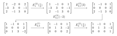
Four matrices connected by arrows show successive row operations producing pivots and zeros below each pivot.
Let $A$ be an $m \times n$ matrix, and let $B = (b_{ij})$ be the result when $\mathsf{Alg1}$ is run on $A$. Show that there exist integers $1 \le n_1 < \cdots < n_k \le n$ with $k \le m$ such that
- (i)
$b_{i n_i} = 1$ for all $1 \le i \le k$, and
- (ii)
$b_{i x} = 0$ when $x < n_i$ or $i > k$.
A matrix in this form is sometimes said to be in row echelon form.
Let $A$ be an $m \times n$ matrix, and let $E$ be an $m \times m$ elementary matrix. Show that $\rank(EA) = \rank(A)$. Conclude that $\rank(A)$ is the number of nonzero rows when $A$ is made into a row echelon form by $\mathsf{Alg1}$.
Actually, we can further simplify the matrix by using the $1$'s we have obtained to cancel out all the terms above it. Consider the following algorithm, which we call $\mathsf{Alg2}$.
- 1.
Start from the second row, with first nonzero entry $a_{2j} = 1$.
- 2.
Cancel out the entry $a_{1j}$ by adding $-a_{1j}$ times the second row to the first row.
- 3.
Move to the next row, whose first nonzero entry is $a_{3j^\prime} = 1$.
- 4.
Again, cancel out the entries $a_{1j^\prime}$ and $a_{2j^\prime}$ by adding the third row times a constant to the first and second rows.
- 5.
Repeat the process until we get to the last nonzero row.
Again, as an example, I have run this algorithm on the result of Figure 3.3 in Figure 3.4.
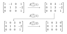
Three matrices connected by arrows show backward elimination and pivot scaling after row echelon form has been reached.
By running $\mathsf{Alg1}$ and $\mathsf{Alg2}$ on the given matrix, I have shown that
$$ \begin{aligned} \begin{bmatrix} 1 & 0 & 3 & 0 \\ 0 & 1 & 3 & 0 \\ 0 & 0 & 0 & 1 \end{bmatrix} &= E_{2,3}^{(3)}(2) \cdot E_{1,3}^{(3)}(1) \cdot E_{1,2}^{(3)}(1) \cdot E_{3}^{(2)}(\tfrac{1}{2}) \\ &\qquad \cdot E_{2,3}^{(1)} \cdot E_{3,1}^{(3)}(-2) \cdot E_{2,1}^{(3)}(3) \cdot E_1^{(2)}(\tfrac{1}{2}) \cdot \begin{bmatrix} 2 & -2 & 0 & 2 \\ -3 & 3 & 0 & -1 \\ 2 & -1 & 3 & 0 \end{bmatrix}. \end{aligned} $$
If we run $\mathsf{Alg1}$ and $\mathsf{Alg2}$ on a square matrix, and the resulting matrix happens to be the identity matrix, then we would get $I = E_1 \cdots E_n \cdot A$, and then $E_1 \cdots E_n$ will be the inverse of $A$.
Let $A$ be an $m \times n$ matrix, and let $B = (b_{ij})$ be the result when $\mathsf{Alg1}$ and then $\mathsf{Alg2}$ are run on $A$. Show that there exist integers $1 \le n_1 < \cdots < n_k \le n$ with $k \le m$ such that
- (i)
$b_{i n_i} = 1$ for $1 \le i \le k$,
- (ii)
$b_{i x} = 0$ for $x < n_i$ or $i > k$, and
- (iii)
$b_{x n_i} = 0$ for $1 \le i \le k$ and $x \neq n_i$.
A matrix in this form is said to be in reduced row echelon form.
Let $A$ be an invertible $n \times n$ matrix. Show that the result of $\mathsf{Alg1}$ and $\mathsf{Alg2}$ run on $A$ is the $n \times n$ identity matrix $I$. Use this to show that the following algorithm calculates the inverse matrix of $A$:
- 1.
First consider the $n \times 2n$ matrix $\tilde{A} = \begin{bmatrix} A & I \end{bmatrix}$ defined by putting the $n \times n$ identity matrix on the right side of $A$.
- 2.
Run $\mathsf{Alg1}$ and then $\mathsf{Alg2}$ on $\tilde{A}$.
- 3.
Discard the first $n$ columns to get an $n \times n$ matrix.
Let $A$ be an invertible $n \times n$ matrix, and let $b \in k^n$ be an $n \times 1$ column vector. Show that the following algorithm solves the equation $Ax = b$:
- 1.
First consider the $n \times (n+1)$ matrix $\tilde{A} = \begin{bmatrix} A & b \end{bmatrix}$ defined by augmenting $A$ with the $n \times 1$ vector $b$ to the right.
- 2.
Run $\mathsf{Alg1}$ and then $\mathsf{Alg2}$ on $\tilde{A}$.
- 3.
Take the $(n+1)$th column.